Transport Correction Ratio Notebook

Return to Transport Correction Ratio documentation.

Transport Correction Ratio

This notebook is used to compare transport correction ratios (TCR) for H-1 and higher atomic mass isotopes.

# import relevant packages
import matplotlib.pyplot as plt
import numpy as np
import pandas as pd
import time
plt.rcParams['font.size'] = 16
plt.rcParams['figure.figsize'] = [6, 4] # Set default figure sizeimport numpy as np

# import relevant functions from transportcorrection.py
from transportcorrection import energyInterpolation, InfFlux, Plot1d, analyticTCR

Read in cross section data

# read in data from desired data file (first we will use H1 data)
data = pd.read_csv("./database/H2.csv")
isotopeMass = 2
isotopeName = "H2"
energy = np.array(data['energy'])
sigT = np.array(data['total'])
sigS = np.array(data['scattering'])

Define the source term

# source term definition
# fission spectrum
srcFiss = np.exp(-energy/9.880E+05)*np.sinh((2.249E-06*energy)**0.5)
srcFiss = srcFiss / np.sum(srcFiss)
# Monoenergetic source
srcMono = np.zeros_like(energy)
srcMono[-1] = energy[-1]
srcMono = srcMono / np.sum(srcMono)

Interpolate the energy and cross section data to improve resolution

energyN = 501 # number of energy points
lowerE, upperE = 1, 19E+06  #  upper and lower energy limits

# Define interpolated arrays for fission spectrum source and monoenergetic source
sigS1Fiss, sigT1Fiss, src1Fiss, energy1Fiss =\
    energyInterpolation(energy, sigS, sigT, srcFiss, energyN, lowerE, upperE,'log')

sigS1Mono, sigT1Mono, src1Mono, energy1Mono =\
    energyInterpolation(energy, sigS, sigT, srcMono, energyN, lowerE, upperE,'log')

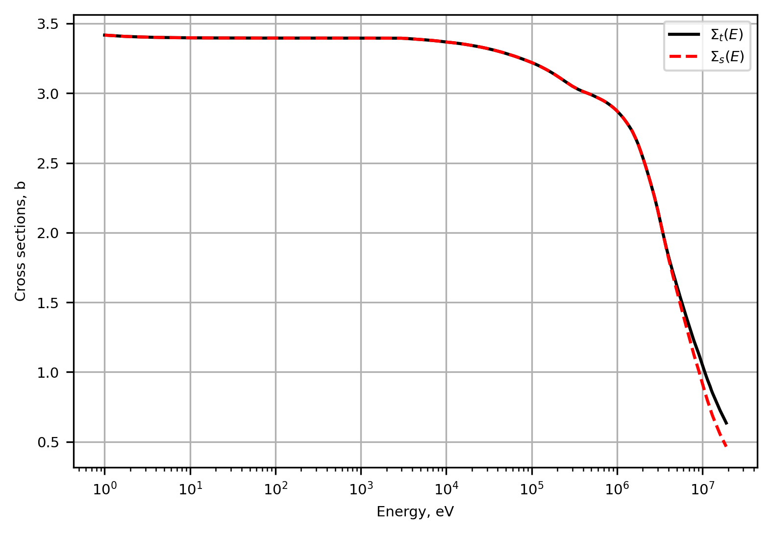
plt.figure()
Plot1d(energy1Fiss, sigT1Fiss, xlabel="Energy, eV", ylabel="total", fontsize=7, marker="-k", markerfill=False, markersize=6, legend="$\Sigma_{t}(E)$")
Plot1d(energy1Fiss, sigS1Fiss, xlabel="Energy, eV", ylabel="Cross sections, b", fontsize=7, marker="--r", markerfill=False, markersize=6, legend="$\Sigma_{s}(E)$")
plt.grid()

Solve for flux using either an infinite flux formulation or a separate analytic flux

Infinite flux general form for A \(\ge\) 1:

\[\begin{equation} \Sigma_T(E)\phi(E)=\int_E^{\infty}\frac{\Sigma_s(E')\phi(E')}{(1-\alpha)E'}dE'+S(E) \end{equation}\]

where \(\alpha\) is:

\[\begin{equation} \alpha = \frac{(1-A)^2}{(1+A)^2} \end{equation}\]

# choose the infinite flux solution (from fission spectrum source or monoenergetic source)
flxFiss = InfFlux(energy1Fiss, sigS1Fiss, sigT1Fiss, src1Fiss, isotopeMass)
flxMono = InfFlux(energy1Mono, sigS1Mono, sigT1Mono, src1Mono, isotopeMass)
# normalized
flxNormFiss = flxFiss/np.sum(flxFiss)
flxNormMono = flxMono/np.sum(flxMono)

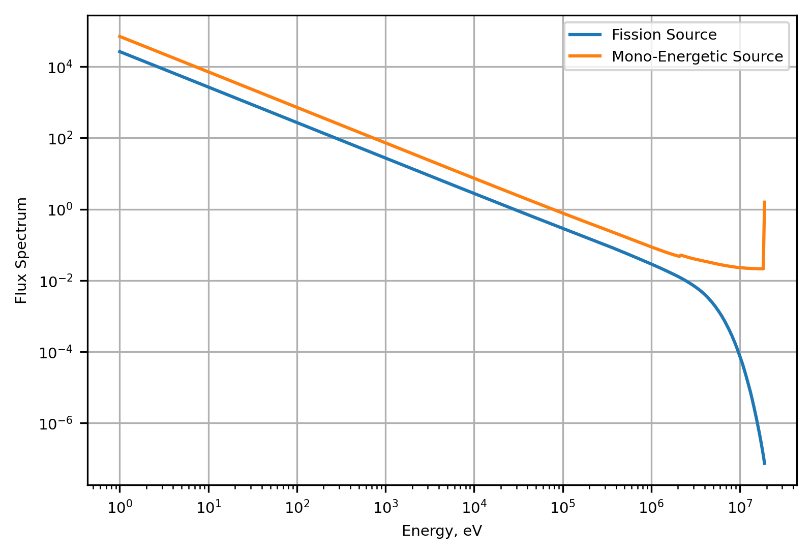
# Plots for comparing mono-energetic to fission sources
plt.figure()
plt.loglog(energy1Fiss, flxFiss, label='Fission Source')
plt.loglog(energy1Mono,flxMono, label='Mono-Energetic Source')
plt.xlabel('Energy, eV'), plt.ylabel('Flux Spectrum'), plt.legend()
plt.grid()

Solve for the TCR using:

\[\begin{equation} \tau(E)=\left[ 1+\frac{1}{\phi(E)} \int_E^{E_{max}} dE'\frac{\phi(E')\mu(E' \rightarrow E)}{\tau(E')(1-\alpha)(E')} \right]^{-1} \end{equation}\]

where

\[\begin{equation} \mu(E' \rightarrow E)= \frac{1}{2}(A+1)\sqrt{\frac{E}{E'}}-\frac{1}{2}(A-1)\sqrt{\frac{E'}{E}} \end{equation}\]

#using simpson method
start=time.time()
tauFissSimpson = analyticTCR(energy1Fiss, flxNormFiss, isotopeMass, 'simpson')
end=time.time()
print(f"calculation took {end-start:.4f}s")

#using trapezoid method
start=time.time()
tauFissTrap = analyticTCR(energy1Fiss, flxNormFiss, isotopeMass, 'trapezoid')
end=time.time()
print(f"calculation took {end-start:.4f}s")

calculation took 0.0715s
calculation took 0.0458s

# find average cosine of the scattering angle and Tau as energy approaches 0
tau0=(1-2/(3*isotopeMass))*np.ones(flxNormFiss.shape[0])

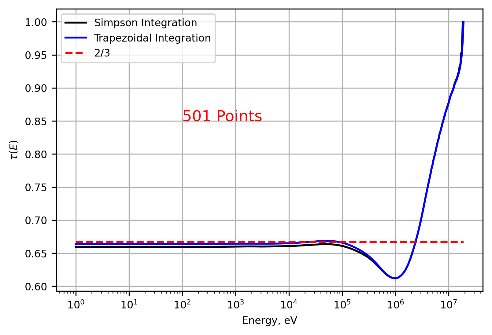
plt.figure()
Plot1d(energy1Fiss, tauFissSimpson, xlabel="Energy, eV", ylabel="$\\tau(E)$", fontsize=8, marker="-k", markerfill=False, markersize=6, legend='Simpson Integration')
plt.grid()
Plot1d(energy1Fiss, tauFissTrap, xlabel="Energy, eV", ylabel="$\\tau(E)$", fontsize=8, marker="-b", markerfill=False, markersize=6, legend='Trapezoidal Integration')
plt.grid()
Plot1d(energy1Fiss, tau0, xlabel="Energy, eV", ylabel="$\\tau(E)$", fontsize=8, marker="--r", markerfill=False, markersize=6, legend=f'{isotopeMass}/3')
plt.text(100, 0.85, "501 Points", fontsize=12, color="r")

Text(100, 0.85, '5001 Points')

diff = np.abs(tauFissSimpson - tauFissTrap)
# Find the index of the maximum difference
max_index = np.argmax(diff)
max_value = diff[max_index]
print(f"Max difference: {max_value}")

Max difference: [0.02935336]