Weighted Delta Tracking Notebook
Return to Weighted Delta Tracking documentation.
# import relevant packages
import matplotlib.pyplot as plt
import numpy as np
plt.rcParams['font.size'] = 16
%matplotlib inline
plt.rcParams['figure.figsize'] = [6, 4] # Set default figure size
Neutron Transport with Monte Carlo
Description
The purpose of this workshop is to implement two techniques that are used in Monte Carlo codes: 1. Surface (ray-tracing) - ST 2. Delta tracking - DT.
Problem set-up
We will have a point source (located at the origin) surrounded with multiple shells of heterogeneous materials having unique cross sections. Our objectives are to calculate the: - Flux distribution, which for simplicity is defined as the neutrons crossing a certain surface - Leakage from the system (i.e., sphere)
Set of exercises
You are required to complete the following exercises: 1. Analytic solution 2. Ray-tracing 3. Delta tracking
Analytic solution
The programming will be done within the pointsource_sphere.py file.
Note that we use object-oriented programming. This is not mandatory and
only done here as a means of demonestration.
Open the file to familiarize yourself with the __init__ method. This
is done together with the lecturer. Note that the entire volume is
divided to equal-volume shells, according to which the corresponding
radii are calculated. Also, the total and absorption cross sections are
identical (i.e., no scattering)
Complete the _Analytic function that enables to calculate the
analytic solution.
The analytic solution can be derived as:
\(\frac{I(R_i)}{I_0}={\prod}_{j=1}^i e^{-\Sigma_{t,j}\Delta R_j}\)
with the leakage calculated when \(i\) represents the last shell (i.e., \(R_{sphere}\))
Import the class:
>>> mc = PointSourceInSphere(nMC, S0, R, sigT)
where, - nMC is the number of Monte Carlo repetitive simulations -
S0 is the number of source neutrons - R is the radius of the
sphere in cm - sigT total cross section array for all the different
regions
results are stored under the resAN, resST, resDT
dictionaries on the created mc object.
Define inputs and execute analytic solution
from pointsource_sphere import PointSourceInSphere
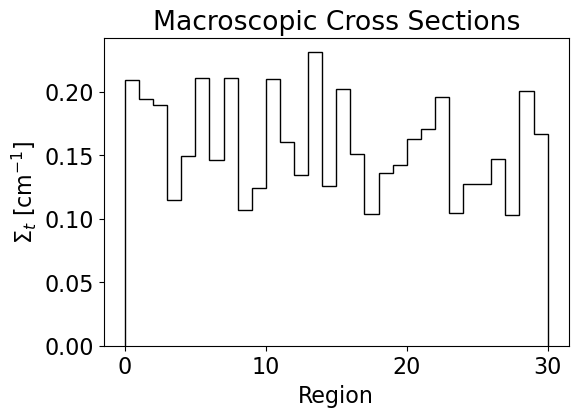
xs = np.random.uniform(low = 0.1, high = 0.25, size = (30))
# xs[6] = 3
mc = PointSourceInSphere(100, 10000, 12.0, xs) # np.full(10, 0.1)
print(xs)
[0.1001577  0.24530646 0.13664874 0.17337634 0.22243201 0.116862
 0.24406138 0.19113768 0.24014224 0.18559167 0.13206509 0.15422328
 0.16250685 0.18396762 0.19339512 0.15167535 0.1241924  0.163639
 0.1427731  0.16122647 0.1301141  0.17603432 0.15403576 0.23975469
 0.13041069 0.23468564 0.22490938 0.17498096 0.12517552 0.1557442 ]
plt.hist(xs, edgecolor = "black")
plt.title("Macroscopic Cross Sections")
plt.xlabel(r"$\Sigma_t$ [cm$^{-1}]$")
plt.ylabel("Count")
plt.show()
mc.Solve('analytic')
mc.resAN
{'flx': array([6792.23679884, 5309.72841784, 4822.63356824, 4375.98125962,
        3938.64253733, 3752.71668664, 3428.67300092, 3215.24031022,
        2985.09278502, 2830.17927413, 2731.55169414, 2627.12087817,
        2527.0093459 , 2423.60282792, 2324.20390758, 2252.32507449,
        2197.4362569 , 2129.81343422, 2074.57290141, 2015.97604744,
        1971.39051637, 1914.44518245, 1867.39692943, 1798.44646182,
        1763.00554365, 1702.58105621, 1648.01216105, 1607.76355352,
        1580.23325575, 1547.39283243]),
 'leakage': np.float64(0.15473928324256722)}
print("Leakage = {:.2f} %".format(100*mc.resAN['leakage']))
Leakage = 15.47 %
# Sanity check
print("Expected leakage = {:.2f} %".format(100*np.exp(-12*0.1)))
Expected leakage = 30.12 %
Ray-tracing
Complete the _SolveST method. Note that the sampling of the point
source should not be performed at all as it is known that all the
neutrons are born in the origin. However, the purpose was to describe
the general sampling approach within the sphere.
Also, all the source neutrons are sampled simultaneously (vectorized) as opposed to one-by-one. The general approach of ST is: 1. Sample \(x_0\), \(y_0\), \(z_0\) 2. Sample distance traveled \(S_i\) 3. Update the position \(x_1\), \(y_1\), \(z_1\) 4. Check if the position is within the shell where the neutrons originated or not - If within the shell, then terminate the neutron - Otherwise, promote the neutron in the same direction to the end of the shell and update \(x_0\), \(y_0\), \(z_0\) and go to step 2. 5. If the neutron crossses the last shell terminate it 6. Our scoring is fairly random here and we will be scoring neutrons that crossed a specific surface. This is easy to do with ST and in this specific case even easier as all the neutrons are traveling in the radial direction only and no scattering events are happening.
Define inputs and execute ST solution
mc.Solve('ST')
mc.resST
{'flx': array([6804.05, 5317.14, 4827.56, 4381.31, 3942.58, 3756.79, 3432.88,
        3219.82, 2990.41, 2835.94, 2738.38, 2635.04, 2534.26, 2431.67,
        2330.14, 2258.55, 2204.37, 2137.71, 2082.44, 2022.84, 1978.08,
        1920.93, 1873.65, 1804.81, 1769.21, 1707.42, 1653.21, 1612.46,
        1583.82, 1551.58]),
 'fluxsim': array([[6756., 6815., 6761., ..., 6846., 6845., 6724.],
        [5268., 5313., 5249., ..., 5289., 5355., 5271.],
        [4789., 4832., 4780., ..., 4838., 4845., 4807.],
        ...,
        [1589., 1604., 1608., ..., 1642., 1667., 1616.],
        [1564., 1573., 1581., ..., 1606., 1635., 1588.],
        [1530., 1540., 1553., ..., 1571., 1597., 1556.]], shape=(30, 100)),
 'errflx': array([43.80670611, 51.39202662, 51.10994424, 48.92171195, 50.00703551,
        48.80169977, 47.64541531, 45.18547997, 43.62570229, 43.09496954,
        41.64823646, 41.34753197, 38.40901457, 38.15024377, 36.75840584,
        35.81741895, 34.97331983, 34.47471392, 34.06649967, 33.67483333,
        33.29765157, 33.24251946, 33.7073805 , 32.34553911, 31.57603363,
        30.75131867, 31.83843432, 32.46980751, 32.36954742, 32.62060085]),
 'leakage': np.float64(0.15515800000000002),
 'errleakage': np.float64(0.0032620600852835305)}
print(np.std(mc.resST['fluxsim'][0]))
print(np.mean(np.abs((mc.resST['flx'])-(mc.resAN['flx'])))/(mc.resAN['flx']))
43.806706107626944
[0.00090125 0.00115289 0.00126933 0.00139889 0.00155422 0.00163122
 0.00178539 0.00190391 0.0020507  0.00216294 0.00224104 0.00233012
 0.00242244 0.00252579 0.00263381 0.00271787 0.00278575 0.0028742
 0.00295074 0.0030365  0.00310518 0.00319754 0.0032781  0.00340378
 0.00347221 0.00359543 0.00371449 0.00380747 0.00387381 0.00395602]
mc.PlotFluxes('ST')
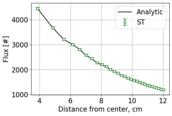
print("Analytic Leakage = {:.2f} %".format(100*mc.resAN['leakage']))
print("MC/ST Leakage = {:.2f} %".format(100*mc.resST['leakage']))
Analytic Leakage = 15.47 %
MC/ST Leakage = 15.52 %
Delta tracking
Complete the _SolveDT method.
The general approach of DT is: 1. Sample \(x_0\), \(y_0\), \(z_0\) 2. Sample virtual distance traveled \(S_i\) using the majorant cross section. 3. Update the position \(x_1\), \(y_1\), \(z_1\) 4. Accept the virtual collision as a real one by sampling uniformly from [0, 1] and comparing to the \(\Sigma_t/\Sigma_{maj}\) - If virtual collision accepted (i.e. a real collision occurred), then terminate the neutron - Otherwise, use the new position as \(x_0\), \(y_0\), \(z_0\) and go to step 2.
Define inputs and execute ST solution
mc.Solve('DT')
mc.resDT
{'flx': array([6794.78, 5308.93, 4818.47, 4372.35, 3936.42, 3750.66, 3428.73,
        3214.5 , 2983.32, 2827.64, 2729.1 , 2625.43, 2527.19, 2422.75,
        2325.28, 2252.2 , 2196.9 , 2130.59, 2075.79, 2017.7 , 1971.81,
        1915.89, 1869.63, 1800.63, 1764.28, 1705.2 , 1649.95, 1609.74,
        1581.72, 1548.59]),
 'fluxsim': array([[6746., 6760., 6883., ..., 6824., 6708., 6823.],
        [5315., 5278., 5401., ..., 5314., 5202., 5318.],
        [4819., 4790., 4889., ..., 4828., 4727., 4811.],
        ...,
        [1610., 1554., 1618., ..., 1656., 1599., 1656.],
        [1577., 1523., 1591., ..., 1620., 1571., 1623.],
        [1546., 1497., 1566., ..., 1579., 1546., 1591.]], shape=(30, 100)),
 'errflx': array([47.50296412, 54.29295627, 52.57593651, 53.3729098 , 51.42337601,
        52.65723502, 54.91627354, 54.30883906, 51.32073265, 49.30345221,
        50.27096578, 46.76991661, 45.77459885, 44.98741491, 44.23642843,
        41.55694888, 40.54910603, 40.6396592 , 41.52090919, 41.10145983,
        41.46581604, 40.55265589, 40.98796287, 40.33872953, 39.57400157,
        38.31083398, 36.95520938, 36.11969546, 35.40567186, 34.75027914]),
 'leakage': np.float64(0.154859),
 'errleakage': np.float64(0.0034750279135569535)}
print(np.std(mc.resDT['fluxsim'][0]))
47.50296411804215
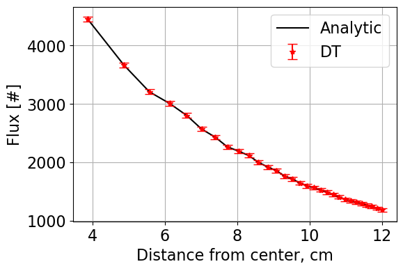
mc.PlotFluxes('DT')
Weighted Delta tracking
mc.Solve('wdt')
mc.resWDT
{'flx': array([6792.04265786, 5314.43065786, 4826.78073402, 4380.50180601,
        3942.89278974, 3756.74802999, 3430.67170231, 3218.33504717,
        2987.87017047, 2832.13629052, 2732.95352074, 2628.11716643,
        2527.24854061, 2424.56506084, 2324.01140579, 2252.26025819,
        2197.08362733, 2129.25424065, 2073.82327713, 2014.78855142,
        1970.59615981, 1913.263707  , 1865.43220038, 1796.47969024,
        1761.59865691, 1700.94228579, 1646.2113917 , 1605.98254835,
        1578.49698119, 1546.47642238]),
 'fluxsim': array([[6719.45389855, 6781.10291923, 6785.46103476, ..., 6788.18245094,
         6795.67208711, 6804.2760478 ],
        [5283.77106551, 5277.35202785, 5291.46172668, ..., 5272.00577991,
         5309.02695805, 5278.16029668],
        [4788.81749607, 4799.64144118, 4814.60293046, ..., 4798.74256932,
         4821.417972  , 4811.50190581],
        ...,
        [1580.76313154, 1613.14782101, 1583.10873522, ..., 1597.10809609,
         1620.43889207, 1574.88283747],
        [1552.86483339, 1589.72048029, 1560.58995791, ..., 1569.10778227,
         1596.70158823, 1547.81930338],
        [1525.21531175, 1554.62002756, 1533.52909093, ..., 1540.42166307,
         1564.4752873 , 1519.56155598]], shape=(30, 100)),
 'errflx': array([34.14347062, 41.12309217, 39.05960755, 38.94947025, 39.56659299,
        38.18744016, 38.49054524, 37.3352865 , 38.41194481, 37.4671756 ,
        36.72014899, 36.69297015, 36.36485655, 34.91086451, 34.49571066,
        33.95676986, 33.12171791, 32.6284291 , 32.45204713, 32.880467  ,
        32.71928672, 32.58150959, 32.1368518 , 31.79327865, 31.2677748 ,
        29.74636004, 28.33795562, 28.49143501, 27.97191187, 27.90330159]),
 'leakage': np.float64(0.1546476422375583),
 'errleakage': np.float64(0.002790330158587489)}
print(np.std(mc.resWDT['fluxsim'][0]))
34.14347061579633
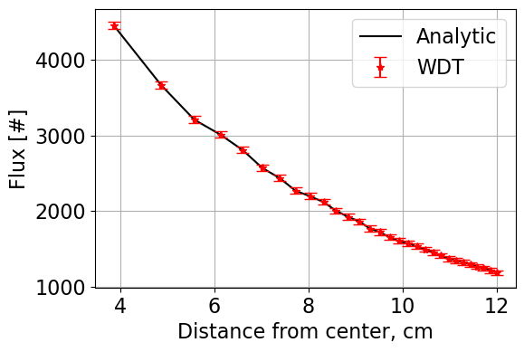
mc.PlotFluxes('WDT')
print("Analytic Leakage = {:.2f} %".format(100*mc.resAN['leakage']))
print("MC/ST Leakage = {:.2f} %".format(100*mc.resST['leakage']))
print("MC/DT Leakage = {:.2f} %".format(100*mc.resDT['leakage']))
print("MC/WDT Leakage = {:.2f} %".format(100*mc.resWDT['leakage']))
Analytic Leakage = 15.47 %
MC/ST Leakage = 15.52 %
MC/DT Leakage = 15.49 %
MC/WDT Leakage = 15.46 %
Execution times
print("ST = {:.2f}".format(mc.times['ST']))
print("DT = {:.2f}".format(mc.times['DT']))
print("WDT = {:.2f}".format(mc.times['WDT']))
ST = 45.28
DT = 23.55
WDT = 32.26
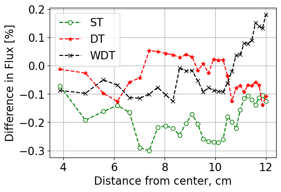
mc.PlotDifferences()
Return to top of notebook: Weighted Delta Tracking Notebook