Fuel Assembly Diffusion
Return to Diffusion Coefficients and Critical Spectrum Search documentation.
# import relevant packages
import numpy as np
from scipy.linalg import solve
import matplotlib.pyplot as plt
from matplotlib import rcParams

# Default values
FONT_SIZE = 16  # font size for plotting purposes
# rcParams['figure.dpi'] = 300
plt.rcParams['figure.figsize'] = [6, 4] # Set default figure size
import serpentTools
from serpentTools.settings import rc
from plotter import Plot1d
from numerical_TCR import InScatter, OutScatter, FluxLimited, Condense2gr
Transport cross section
Description
In-scatter
\(\Sigma_{tr,g} = \Sigma_{t,g} - \frac{{\sum}_{g'}\Sigma_{s1,g'g}J_{g'}}{J_g}\)
Out-scatter
\(\Sigma_{tr,g} \approx \Sigma_{t,g} - \frac{{\sum}_{g'}\Sigma_{s1,gg'}J_{g}}{J_g}=\Sigma_{t,g}-\Sigma_{s1,g}\)
Flux-limited
\(\Sigma_{tr,g} = \Sigma_{t,g} - \frac{{\sum}_{g'}\Sigma_{s1,g'g}\phi_{g'}}{\phi_g}\)
Obtain the current
\(\Sigma_{t,h}J_h-{\sum}_{h'}\Sigma_{s1,h'h}J_{h'}=\frac{1}{3}B\phi_h\)
Read results from Serpent
# 70-group Infinite Results
resFile70gr = "./serpent/fa2D_70gr_inf_res.m"
# 2-Group B1 Leakage Corrected Reference Results
resFile2gr = "./serpent/fa2D_2gr_B1_res.m"
# 70-group Infinite Hydrogen Results
resFile70grH = "./serpent/infinite_h_basic_h1_r1_res.m"
# Read the results using the serpentTools package
rc["serpentVersion"] = "2.2.1"
res70gr = serpentTools.read(resFile70gr)
res2gr = serpentTools.read(resFile2gr)
res70grH = serpentTools.read(resFile70grH)
SERPENT Serpent 2.1.32 found in ./serpent/infinite_h_basic_h1_r1_res.m, but version 2.2.1 is defined in settings
  Attempting to read anyway. Please report strange behaviors/failures to developers.
# 70-group fuel assembly data
ng = 70
univ0 = res70gr.getUniv('0', timeDays=0)
flxLat = univ0.infExp['infFlx']
sigTLat = univ0.infExp['infTot']
SP1Lat = univ0.infExp['infSp1']
cmmTranspLat = univ0.gc['cmmTranspxs']      # represents in-scatter
infTranspLat = univ0.infExp['infTranspxs']  # out-scatter
energyLat = univ0.groups * 1e6
# Retrieve the reference diffusion coefficients for 2-groups
univ0 = res2gr.getUniv('0', timeDays=0)
cmmDiffCoeff2g = univ0.gc['cmmDiffcoef']
# using the serpent results to get infinite TCR
cmmTauLat = cmmTranspLat / sigTLat
To create the scattering matrix with the following structure: 1->1, 2->1 3->1 … 1->2, 2->2 3->2 … 1->3, 2->3 3->3 … …
SP1Lat=SP1Lat.reshape((ng,ng)).transpose()
Execute in-scatter function
inSigTrLat, inTauLat, JgLat = InScatter(ng, SP1Lat, sigTLat, flxLat, B2=1E-06)
Execute the out-scatter
outSigTrLat, outTauLat = OutScatter(ng, SP1Lat, sigTLat)
Execute the flux-limited
limitSigTrLat, limitTauLat = FluxLimited(ng, SP1Lat, sigTLat, flxLat)
A 2-group energy structure is defined for fast and thermal neutrons with group 1 (fast) having energies > 0.625 eV and group 2 (thermal) having energies \(\le\) 0.625 eV.
# Find the energy cutoff index
energyCutoff = 0.625 # energy cutoff value defining neutron energy group [eV]
g1Indices = np.where(energyLat > 0.625)[0]
g2Indices = np.where(energyLat <= 0.625)[0]
Diffusion Coefficient Group Condensation
Determine the 2-group diffusion coefficients for in-scatter, out-scatter, and flux-limited defined transport cross sections.
inDiffCoeff2g = Condense2gr(1/(3*inSigTrLat), flxLat, energyLat, cutoffE=0.625)
outDiffCoeff2g = Condense2gr(1/(3*outSigTrLat), flxLat, energyLat, cutoffE=0.625)
limitDiffCoeff2g = Condense2gr(1/(3*limitSigTrLat), flxLat, energyLat, cutoffE=0.625)
print(f"The 2-group diffusion coefficients for the in-scatter method are {inDiffCoeff2g} with relative errors of {100*(inDiffCoeff2g-cmmDiffCoeff2g)/cmmDiffCoeff2g}%.")
print(f"The 2-group diffusion coefficients for the out-scatter method are {outDiffCoeff2g} with relative errors of {100*(outDiffCoeff2g-cmmDiffCoeff2g)/cmmDiffCoeff2g}%.")
print(f"The 2-group diffusion coefficients for the flux-limited method are {limitDiffCoeff2g} with relative errors of {100*(limitDiffCoeff2g-cmmDiffCoeff2g)/cmmDiffCoeff2g}%.")
The 2-group diffusion coefficients for the in-scatter method are [1.69854949 0.88303605] with relative errors of [-3.38501006 -0.56684185]%.
The 2-group diffusion coefficients for the out-scatter method are [1.73376106 0.82629467] with relative errors of [-1.38214492 -6.95613244]%.
The 2-group diffusion coefficients for the flux-limited method are [1.68208348 0.87193724] with relative errors of [-4.32161155 -1.8166092 ]%.
Read 70-group data from infinite hydrogen assembly to perform hydrogen correction for out-scatter calculated \(\Sigma_{tr}\)
univ0 = res70grH.getUniv('0', timeDays=0)
flxH = univ0.infExp['infFlx']
sigTH = univ0.infExp['infTot']
SP1H = univ0.infExp['infSp1']
cmmTranspH = univ0.gc['cmmTranspxs']      # represents in-scatter
infTranspH = univ0.infExp['infTranspxs']  # out-scatter
energyH = univ0.groups * 1e6
SP1H=SP1H.reshape((ng,ng)).transpose()

# Calculate the in-scatter method transport correction factor for H-1
inSigTrH, inTauH, JgH  = InScatter(ng, SP1H, sigTH, flxH, B2=1E-04)

# Calculate the microscopic transport cross section using out-scatter macroscopic transport cross section
outSigTrH, outTauH = OutScatter(ng, SP1H, sigTH)
numberDensInf = 4.29318E+23 # from N = rho*Avagadro/(mass_H)
outMicroTrH = infTranspH/numberDensInf

# Remove the hydrogen generated transport xs from the lattice transport xs
numberDensLat = 2.7496E+22 # hydrogen number density smeared over lattice
outSigTrLatMinus = infTranspLat - outMicroTrH * numberDensLat

# Find microscopic total cross section for hydrogen
microTotalH = sigTH/numberDensInf
outSigTrLatCorrected = outSigTrLatMinus + microTotalH * numberDensLat * inTauH
Calculate the corrected 2-group diffusion coefficients for the out-scatter method
outDiffCoeff2gCorrected = Condense2gr(1/(3*outSigTrLatCorrected), flxLat, energyLat, cutoffE=0.625)
print(f"The 2-group diffusion coefficients for the corrected out-scatter method are {outDiffCoeff2gCorrected} with relative errors of {100*(outDiffCoeff2gCorrected-cmmDiffCoeff2g)/cmmDiffCoeff2g}%.")
The 2-group diffusion coefficients for the corrected out-scatter method are [1.71873483 0.8845672 ] with relative errors of [-2.23685006 -0.3944285 ]%.
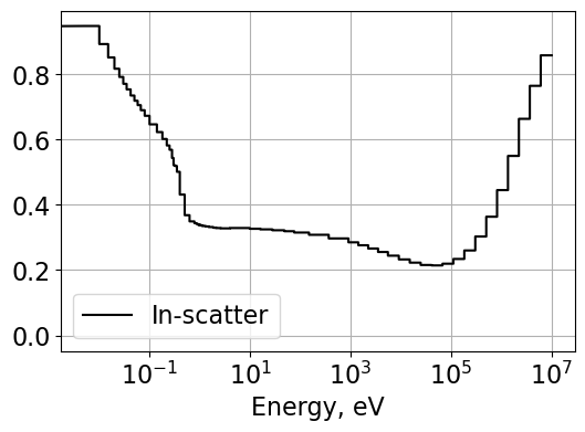
# Plot in-scatter TCR used for hydrogen correction
plt.figure()
Plot1d(energyH, inTauH, xlabel="Energy, eV", ylabel='',
        fontsize=16, marker="-k", markerfill=False, markersize=6)
plt.legend(['In-scatter'])
<matplotlib.legend.Legend at 0x2f60c037950>
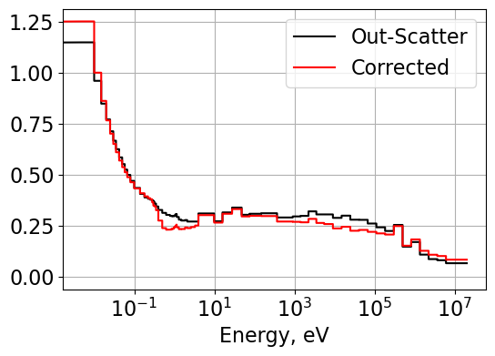
# Plot hydrogen corrected out-scatter transport cross sections
plt.figure()
plt.grid(visible=True)
Plot1d(energyLat, outSigTrLat, xlabel="Energy, eV", ylabel='',
        fontsize=16, marker="-k", markerfill=False, markersize=6)
Plot1d(energyLat, outSigTrLatCorrected, xlabel="Energy, eV", ylabel='',
        fontsize=16, marker="-r", markerfill=False, markersize=6)
plt.legend(['Out-Scatter', 'Corrected'])
<matplotlib.legend.Legend at 0x2f60dfd2590>