Critical Spectrum Calculations

Return to Diffusion Coefficients and Critical Spectrum Search documentation.

import matplotlib.pyplot as plt
from matplotlib import rcParams
# Default values
FONT_SIZE = 16  # font size for plotting purposes
# rcParams['figure.dpi'] = 300
plt.rcParams['figure.figsize'] = [6, 4] # Set default figure size

import numpy as np
import serpentTools
from scipy.linalg import solve
from plotter import Plot1d
from critical_spectrum import SolveB1, SolveCM, CriticalSpectrum, Condense2gr

The \(B_1\) Critical spectrum

\[\begin{split}\begin{equation} \begin{split} \Sigma_{t,g}\phi_g-{\sum}_{g'}\Sigma_{s0,g'g}\phi_{g'}\pm iBJ_g=\chi_g \\ 3a_g(B)\Sigma_{t,g}J_g-3{\sum}_{g'}\Sigma_{s1,g'g}J_{g'}=\mp iB\phi_g \end{split} \end{equation}\end{split}\]

Read results from Serpent

resFile70gr = "./serpent/fa2D_70gr_inf_res.m"
resFile2gr = "./serpent/fa2D_2gr_B1_res.m"

Two-group results [reference point]

res2gr = serpentTools.read(resFile2gr)
univ = res2gr.getUniv('0', timeDays=0)
b1Transp_2gr = univ.b1Exp['b1Transpxs']
b1Rabsxs_2gr = univ.b1Exp['b1Rabsxs']
infTransp_2gr = univ.infExp['infTranspxs']
infRabsxs_2gr = univ.infExp['infRabsxs']
infDiff_2gr = 1/(3*infTransp_2gr)
b1Diff_2gr = 1/(3*b1Transp_2gr)

SERPENT Serpent 2.2.1 found in ./serpent/fa2D_2gr_B1_res.m, but version 2.1.31 is defined in settings
  Attempting to read anyway. Please report strange behaviors/failures to developers.

70-group results

# Read the results using the serpentTools package
res70gr = serpentTools.read(resFile70gr)

SERPENT Serpent 2.2.1 found in ./serpent/fa2D_70gr_inf_res.m, but version 2.1.31 is defined in settings
  Attempting to read anyway. Please report strange behaviors/failures to developers.

ng = 70  # number of energy groups
univ0 = res70gr.getUniv('0', timeDays=0)
flx = univ0.infExp['infFlx']
sigT = univ0.infExp['infTot']
rabsxs = univ0.infExp['infRabsxs']
nusigF = univ0.infExp['infNsf']
chi = univ0.infExp['infChit']
SP1 = univ0.infExp['infSp1']
SP0 = univ0.infExp['infSp0']
cmmTransp = univ0.gc['cmmTranspxs']  # represents in-scatter
infTransp = univ0.infExp['infTranspxs']  # out-scatter
energy = univ0.groups * 1E+06
kinf = res70gr.resdata['absKeff'][0]  # k-inf

To create the scattering matrix with the following structure: 1->1, 2->1 3->1 … 1->2, 2->2 3->2 … 1->3, 2->3 3->3 … …

SP1=SP1.reshape((ng,ng)).transpose()
SP0=SP0.reshape((ng,ng)).transpose()

Solving \(B_1\) equations with a known \(\alpha_g\) and \(B^2\)

From the second \(B_1\) equation a relation between \(J\) and \(\phi\) is established.

\(\pm iB \vec{J} = B^2 \mathbf{D} \vec{\phi}\)

Components of the inverse of D are:

\(D_{gg'}^{-1}=3\alpha_g\Sigma_{t,g}\delta_{gg'}-3\Sigma_{s1,g'g}\)

\(\vec{\phi} = \mathbf{A}^{-1}~\vec{\chi}\)

where, the components of matrix \(A\) are:

\(A_{gg'}=\Sigma_{t,g}\delta_{gg'}-\Sigma_{s0,g'g}+B^2D_{gg'}\)

Solve \(B_1\)

Methodology to iterate on \(B_1\)

\(B^2\)=0 is used to obtain the infinite-medium \(k_{\infty}\) and its associated spectrum. Serpent provide \(k_{\infty}\).
A perturbed value \(B^2=0.0001\) is used to solve for the flux and current.

\[\begin{equation} \begin{split} \frac{k_{\infty}}{M^2}=\frac{B^2(k_1)}{\frac{1}{k_1}-\frac{1}{k_{\infty}}} \end{split} \end{equation}\]

\[\begin{equation} \begin{split} B_1^2(k=1)=B^2(k_1)+\frac{k_{\infty}}{M^2}(\underbrace{1}_{k_{eff}=1}-\frac{1}{k_1}) \end{split} \end{equation}\]

The coefficient \(\frac{k_{\infty}}{M^2}\) is evaluated only once.

\[\begin{equation} \begin{split} D_g=\frac{\pm iJ_g}{B_1\phi_g} \end{split} \end{equation}\]

Energy condensation

\[\begin{equation} \begin{split} D_G=\frac{\sum_{g \in G}D_g\phi_g}{\sum_{g \in G}\phi_g} \end{split} \end{equation}\]

\[\begin{equation} \begin{split} \Sigma_G=\frac{\sum_{g \in G}\Sigma_g\phi_g}{\sum_{g \in G}\phi_g} \end{split} \end{equation}\]

Execute the entire sequence

crit_flxB1, crit_iJB1, B2B1, iB1 = CriticalSpectrum(ng, SP0, SP1, sigT, cmmTransp, chi, nusigF, kinf, P1=False, CM=False)
crit_flxP1, crit_iJP1, B2P1, iP1 = CriticalSpectrum(ng, SP0, SP1, sigT, cmmTransp, chi, nusigF, kinf, P1=True, CM=False)
crit_flxCM, B2CM, iCM= CriticalSpectrum(ng, SP0, SP1, sigT, cmmTransp, chi, nusigF, kinf, P1=False, CM=True)

print(f"The critical B^2 values are B1:{B2B1:.6f}, P1:{B2P1:.6f}, CM:{B2CM:.6f}.")
print(f"k_inf = 1 +/- 1e-6 was achieved in B1:{iB1} iterations, P1:{iP1} iterations, and CM:{iCM} iterations.")

The critical B^2 values are B1:0.000255, P1:0.000254, CM:0.000246.
k_inf = 1 +/- 1e-6 was achieved in B1:4 iterations, P1:3 iterations, and CM:3 iterations.

normFlx = flx / flx.sum()
normFlxCM = crit_flxCM / crit_flxCM.sum()
normFlxB1 = crit_flxB1 / crit_flxB1.sum()
normFlxP1 = crit_flxP1 / crit_flxP1.sum()
flx_diff = 100*(1-normFlx/normFlxB1)

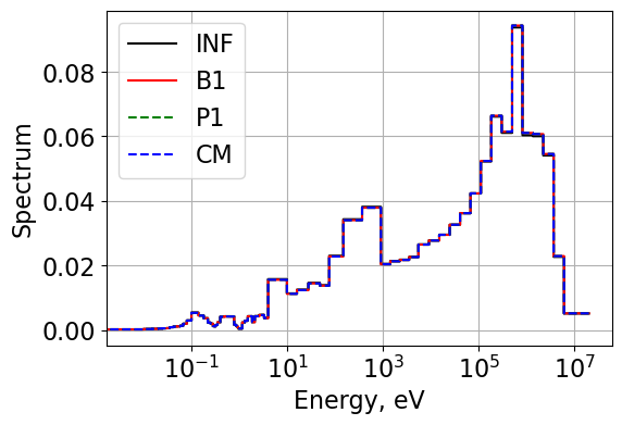
Compare the flux and current spectrum

plt.figure()
plt.grid(visible=True)
Plot1d(energy, normFlx, xlabel="Energy, eV", ylabel='',
        fontsize=16, marker="-k", markerfill=False, markersize=4)
Plot1d(energy, normFlxB1, xlabel="Energy, eV", ylabel='Spectrum',
        fontsize=16, marker="-r", markerfill=False, markersize=6)
Plot1d(energy, normFlxP1, xlabel="Energy, eV", ylabel='Spectrum',
        fontsize=16, marker="--g", markerfill=False, markersize=6)
Plot1d(energy, normFlxCM, xlabel="Energy, eV", ylabel='Spectrum',
        fontsize=16, marker="--b", markerfill=False, markersize=4)
plt.legend(['INF', 'B1',"P1",'CM'])

<matplotlib.legend.Legend at 0x215bd737190>

Diffusion coefficients

# Use eq. 8.21 to obtain the diffusion coefficient
DgB1 = (crit_iJB1) / (crit_flxB1 * B2B1**0.5)
DgP1 = (crit_iJP1) / (crit_flxP1 * B2P1**0.5)

# Note that the diffusion coefficients used in the CM method are calculated using cmmTransport cross sections from Serpent output

Condense into 2-group

\[\begin{equation} \begin{split} D_G=\frac{\sum_{g \in G}D_g\phi_g}{\sum_{g \in G}\phi_g} \end{split} \end{equation}\]

pred_b1Rabsxs_2gr = Condense2gr(rabsxs, crit_flxB1, energy, cutoffE=0.625)
pred_b1Diff_2gr = Condense2gr(DgB1, crit_flxB1, energy, cutoffE=0.625)
pred_p1Rabsxs_2gr = Condense2gr(rabsxs, crit_flxP1, energy, cutoffE=0.625)
pred_p1Diff_2gr = Condense2gr(DgP1, crit_flxP1, energy, cutoffE=0.625)
pred_cmRabsxs_2gr = Condense2gr(rabsxs, crit_flxCM, energy, cutoffE=0.625)
pred_cmDiff_2gr = Condense2gr(1/(3*cmmTransp), crit_flxCM, energy, cutoffE=0.625)
print(f"B1 (Serpent, Reference) results, Dg: {b1Diff_2gr}, Rabsxs: {b1Rabsxs_2gr}.")
print(f"B1 2-group results, Dg: {pred_b1Diff_2gr}, Rabsxs: {pred_b1Rabsxs_2gr}.")
print(f"P1 2-group results, Dg: {pred_p1Diff_2gr}, Rabsxs: {pred_p1Rabsxs_2gr}.")
print(f"CM 2-group results, Dg: {pred_cmDiff_2gr}, Rabsxs: {pred_cmRabsxs_2gr}.")

B1 (Serpent, Reference) results, Dg: [1.69958768 0.88299987], Rabsxs: [0.00775962 0.0676255 ].
B1 2-group results, Dg: [1.69905265 0.88293977], Rabsxs: [0.00776182 0.06764274].
P1 2-group results, Dg: [1.70307681 0.88330774], Rabsxs: [0.00776193 0.06764278].
CM 2-group results, Dg: [1.76303046 0.88447132], Rabsxs: [0.00776121 0.0676434 ].